Viscoelasticity
It is found that for some polymeric materials, such as silly putty and wood, it takes some time for them to respond to an applied stress. This behaviour is time dependent.
We have encountered the linear elastic behaviour for solids with Young’s modulus,
\[ \sigma = E \varepsilon \]
or with shear modulus,
\[ \tau = G\gamma \]
Now we introduce the elastic behaviour for a Newtonian fluid (which comes from the modified version of Newton's second law), where the shear strain rate, \( \frac{{\rm{d}\gamma }}{{\rm{d}}t} \) is proportional to the applied stress, \( \tau \), with a constant of proportionality called viscosity, \( \eta \),
\[ \tau = \eta \frac{{\rm{d}\gamma }}{{\rm{d}}t} \]
At higher temperatures, molecular motion is easier, so the viscosity is temperature dependent,
\[ \eta = {\eta _0}\ {\rm{exp}}\left( {\frac{Q}{{RT}}} \right) \]
Note the fluid elastic behaviour is time dependent, where solid elastic behaviour is time independent.
It is found that many polymeric organic biomaterials, such as wood, have a mixture of these behaviours, called viscoelasticity. This time dependent elastic behaviour can be modelled using Maxwell’s model.
Here, the linear-elastic solid is modelled as a spring:
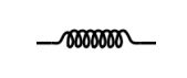
\[ \sigma = k{\varepsilon_{\rm{s}}} \]
and the ideal Newtonian fluid as a dashpot:
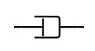
\[ \sigma = \eta \frac{{\rm{d}\varepsilon{_{\rm{l}}}}}{{\rm{d}}t} \]
A spring can store energy when compressed, whereas a dashpot absorbs energy.
In Maxwell’s model, a spring and a dashpot are in series:
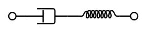
Stresses are equal for components in series and the strains and strain rates can be added,
\[ \varepsilon = { \varepsilon_{\rm{l}}} + { \varepsilon_{\rm{s}}} \]
\[ \dot \varepsilon = {\dot \varepsilon{_{\rm{l}}}} + {{\dot\varepsilon_{\rm{s}}}} \]
\[ \dot \varepsilon = \frac{\sigma }{\eta } + \frac{{\dot \sigma }}{k} \]
\[ k\dot\varepsilon = \frac{k}{\eta }\sigma + \dot \sigma \]
\[ k\dot\varepsilon = \frac{1}{{{t_{\rm{R}}}}}\sigma + \dot \sigma \]
where we let \( {t_{\rm{R}}} = \frac{\eta }{k} \), which is also known as the characteristic relaxation time.
We impose an oscillating stress, which produces a (not necessarily in-phase) strain,
\[ \sigma = {\sigma _0}\exp \left( {i\omega t} \right) \]
\[ \varepsilon = {\varepsilon_0}{\rm{exp}} \left( {i\omega t + \phi } \right) \]
where \( \omega \) is the angular frequency, indicating how frequently the stress and strain oscillate.
Solving the differential equation yields elastic modulus, \( E \) as,
\[ E = \frac{{k{\omega ^2}t_{\rm{R}}^2}}{{1 + {\omega ^2}t_{\rm{R}}^2}} \]
and phase difference, \( \phi \) as,
\[ {\rm{tan}}\phi = \frac{1}{{\omega {t_{\rm{R}}}}} \]
Therefore, a more quantitative description of viscoelasticity using Maxwell’s model is as follows.
High frequencies \( (\omega {t_{\rm{R}}} \) >> 1): phase difference \( \phi \) tends to 0, and there is no delay in the strain response to applied stress. The material behaves like a linear-elastic solid.
Low frequencies \( (\omega {t_{\rm{R}}} \) << 1): phase difference \( \phi \) tends to \( \frac{\pi }{2} \), and elastic modulus E tends to \( k{\omega ^2}t_{\rm{R}}^2 \) and thus to 0. The material behaves like a Newtonian liquid.
Intermediate frequencies \( (\omega {t_{\rm{R}}} \sim 1) \): Stress and strain are out of phase by an intermediate amount. The material behaves like a solid in the sense that the strain is recovered each cycle, but energy is dissipated.
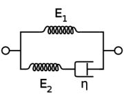
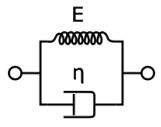
The Maxwell model does not adequately describe the response when subjected to a constant stress. The Voigt model is better at describing this behaviour, with some time dependence and strain tending to a maximum constant value (controlled by the spring).
A clear problem with the Voigt model is that it doesn’t work well at high frequency (the stiffness becomes very large, dominated by the dashpot). A solution to this is the standard linear solid model.